Conduct Physical Simulation
The GIF image above nicely simulates a piece of cloth falling onto a sphere. The cloth in the image is modeled as a mass-spring system, which contains over 10,000 mass points and around 100,000 springs. To simulate a massive physical system at this scale and render it in real-time is never an easy task.
With Taichi, physical simulation programs can be much more readable and intuitive, while still achieving performance comparable to that of C++ or CUDA. With Taichi, those with basic Python programming skills can write high-performance parallel programs in much fewer lines than before, focusing on the higher-level algorithms per se and leaving tasks like performance optimization to Taichi.
In this document, we will walk you through the process of writing a Python program simulating and rendering a piece of cloth falling onto a sphere. Before you proceed, please take a guess of how many lines of code this program consists of.
Get started
Before using Taichi in your Python program, you need to import Taichi to your namespace and initialize Taichi:
- Import Taichi:
import taichi as ti
- Initialize Taichi:
# Choose any of the following backend when initializing Taichi
# - ti.cpu
# - ti.gpu
# - ti.cuda
# - ti.vulkan
# - ti.metal
# - ti.opengl
ti.init(arch=ti.cpu)
We choose ti.cpu here despite the fact that running Taichi on a GPU backend can be much faster. This is mainly because we need to make sure that you can run our source code without any editing or additional configurations to your platform. Please note:
- If you choose a GPU backend, for example
ti.cuda, ensure that you have installed it on your system; otherwise, Taichi will raise an error. - The GGUI we use for 3D rendering only supports CUDA and Vulkan, and x86 for now. If you choose a different backend, consider switching the GGUI system we provide in the source code.
Modelling
This section does the following:
- Generalizes and simplifies the models involved in the cloth simulation.
- Represents the falling cloth and the ball with the data containers provided by Taichi.
Model simplification
This section generalizes and simplifies the models involved in the cloth simulation.
Cloth: a mass-spring system
In this program, the falling cloth is modeled as a mass-spring system. More specifically, we represent the piece of cloth as an n × n grid of mass points, where adjacent points are linked by springs. The following image provided by Matthew Fisher illustrates this structure, where the red vertices are the mass points and the white edges of the grids are the springs.
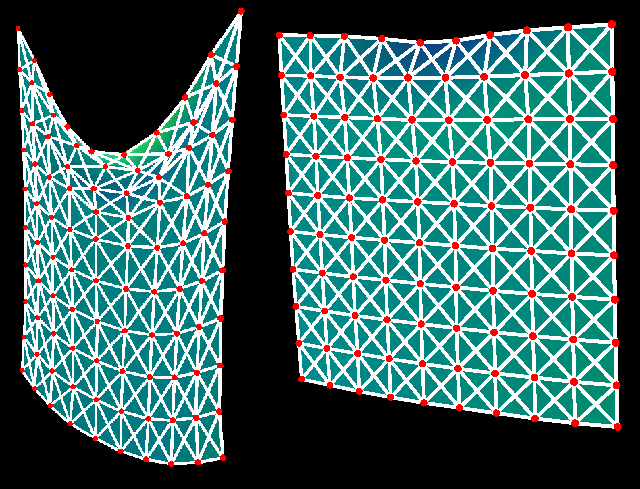
This mass-spring system can be represented by two arrays:
- An n × n array of mass points' positions,
- An n × n array of mass points' velocities.
Further, the position and movement of this system is affected by four factors:
- Gravity
- Internal forces of the springs
- Damping
- Collision with the ball in the middle
Our simulation begins at time t = 0 and advances time by a small constant dt. At the end of each time step dt, the program does the following:
- Estimates the effects of the four factors above on the mass-spring system,
- Updates the position and velocity of each mass point accordingly.
Representation of the ball
A ball can usually be represented by its ball center and radius.
Data structures
In this program, we represent the falling cloth and the ball with the data containers provided by Taichi.
Data structures for cloth
Having initialized Taichi, you can declare the data structures that represent the cloth.
- Declare two arrays
xandvfor storing the mass points' positions and velocities. In Taichi, such arrays are called fields.
n = 128
# x is an n x n field consisting of 3D floating-point vectors
# representing the mass points' positions
x = ti.Vector.field(3, dtype=float, shape=(n, n))
# v is an n x n field consisting of 3D floating-point vectors
# representing the mass points' velocities
v = ti.Vector.field(3, dtype=float, shape=(n, n))
- Initialize the defined fields
xandv:
# The n x n grid is normalized
# The distance between two x- or z-axis adjacent points
# is 1.0 / n
quad_size = 1.0 / n

# The @ti.kernel decorator instructs Taichi to
# automatically parallelize all top-level for loops
# inside initialize_mass_points()
@ti.kernel
def initialize_mass_points():
    # A random offset to apply to each mass point
    random_offset = ti.Vector([ti.random() - 0.5, ti.random() - 0.5]) * 0.1

    # Field x stores the mass points' positions
    for i, j in x:
        # The piece of cloth is 0.6 (y-axis) above the original point
        #
        # By taking away 0.5 from each mass point's [x,z] coordinate value
        # you move the cloth right above the original point
        x[i, j] = [
            i * quad_size - 0.5 + random_offset[0], 0.6,
            j * quad_size - 0.5 + random_offset[1]
        ]
        # The initial velocity of each mass point is set to 0
        v[i, j] = [0, 0, 0]
Data structures for ball
Here, the ball center is a 1D field, whose only element is a 3-dimensional floating-point vector.
ball_radius = 0.3
# Use a 1D field for storing the position of the ball center
# The only element in the field is a 3-dimentional floating-point vector
ball_center = ti.Vector.field(3, dtype=float, shape=(1, ))
# Place the ball center at the original point
ball_center[0] = [0, 0, 0]
Simulation
At the end of each time step dt, the program simulates the effects of the aforementioned four factors on the mass-spring system. In this case, a kernel function substep() is defined.
# substep() works out the *accumulative* effects
# of gravity, internal force, damping, and collision
# on the mass-spring system
@ti.kernel
def substep():
Gravity
# Gravity is a force applied in the negative direction of the y axis,
# and so is set to [0, -9.8, 0]
gravity = ti.Vector([0, -9.8, 0])

# The @ti.kernel decorator instructs Taichi to
# automatically parallelize all top-level for loops
# inside substep()
@ti.kernel
def substep():
    # The for loop iterates over all elements of the field v
    for i in ti.grouped(x):
        v[i] += gravity * dt
note
for i in ti.grouped(x) is an important feature of Taichi. It means that this for loop automatically traverses all the elements of x as a 1D array regardless of its shape, sparing you the trouble of writing multiple levels of for loops.
Either for i in ti.grouped(x) or for i in ti.grouped(v) is fine here because field x has the same shape as field v.
Internal forces of the springs
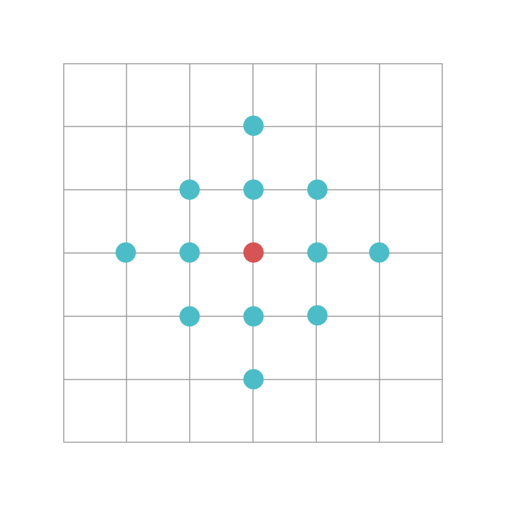
As the image below shows, we make the following assumptions:
- A given point can be influenced by at most 12 neighboring points, and influences from other mass points are neglected.
- These neighboring points exert internal forces on the point through springs.
note
The internal forces here broadly refer to the internal force caused by the elastic deformation of springs and the damping caused by the relative movement of two points.
The code below does the following:
- Traverses the mass-spring grid,
- Accumulates the internal forces that the neighboring points exert on each mass point,
- Translates the internal forces to velocities.
quad_size = 1.0 / n
# Elastic coefficient of springs
spring_Y = 3e4
# Damping coefficient caused by
# the relative movement of the two mass points
# The assumption here is:
# A mass point can have at most 12 'influential` points
dashpot_damping = 1e4

# The cloth is modeled as a mass-spring grid. Assume that:
# a mass point, whose relative index is [0, 0],
# can be affected by at most 12 surrounding points
#
# spring_offsets is such a list storing
# the relative indices of these 'influential' points
spring_offsets = []
for i in range(-1, 2):
    for j in range(-1, 2):
        if (i, j) != (0, 0):
            spring_offsets.append(ti.Vector([i, j]))

@ti.kernel
def substep():

    # Traverses the field x as a 1D array
    #
    # The `i` here refers to the *absolute* index
    # of an element in the field x
    #
    # Note that `i` is a 2-dimentional vector here
    for i in ti.grouped(x):
        # Initial force exerted to a specific mass point
        force = ti.Vector([0.0, 0.0, 0.0])
        # Traverse the surrounding mass points
        for spring_offset in ti.static(spring_offsets):
            # j is the *absolute* index of an 'influential' point
            # Note that j is a 2-dimensional vector here
            j = i + spring_offset
            # If the 'influential` point is in the n x n grid,
            # then work out the internal force that it exerts
            # on the current mass point
            if 0 <= j[0] < n and 0 <= j[1] < n:
                # The relative displacement of the two points
                # The internal force is related to it
                x_ij = x[i] - x[j]
                # The relative movement of the two points
                v_ij = v[i] - v[j]
                # d is a normalized vector (its norm is 1)
                d = x_ij.normalized()
                current_dist = x_ij.norm()
                original_dist = quad_size * float(i - j).norm()
                # Internal force of the spring
                force += -spring_Y * d * (current_dist / original_dist - 1)
                # Continues to apply the damping force
                # from the relative movement
                # of the two points
                force += -v_ij.dot(d) * d * dashpot_damping * quad_size

        # Continues to add the velocity caused by the internal forces
        # to the current velocity
        v[i] += force * dt
Damping
In the real world, when springs oscillate, the energy stored in the springs dissipates into the surrounding environment as the oscillations die away. To capture this effect, we slightly reduce the magnitude of the velocity of each point in the grid at each time step:
# Damping coefficient of springs
drag_damping = 1

@ti.kernel
def substep():

    # Traverse the elements in field v
    for i in ti.grouped(x):
        v[i] *= ti.exp(-drag_damping * dt)
Collision with the ball
We assume that the collision with the ball is an elastic collision: When a mass point collides with the ball, its velocity component on the normal vector of that collision point changes.
Note that the position of each mass point is updated using the velocity at the end of each time step.
# Damping coefficient of springs
drag_damping = 1

@ti.kernel
def substep():

    # Traverse the elements in field v
    for i in ti.grouped(x):

        offset_to_center = x[i] - ball_center[0]
        if offset_to_center.norm() <= ball_radius:
            # Velocity projection
            normal = offset_to_center.normalized()
            v[i] -= min(v[i].dot(normal), 0) * normal
        # After working out the accumulative v[i],
        # work out the positions of each mass point
        x[i] += dt * v[i]
And that's it! This is all the code required to perform a parallel simulation of a mass-spring grid system.
Rendering
We use Taichi's GPU-based GUI system (also known as GGUI) for 3D rendering. GGUI supports rendering two types of 3D objects: triangle meshes and particles. In this case, we can render the cloth as a triangle mesh and the ball as a particle.
GGUI represents a triangle mesh with two Taichi fields: vertices and indices. The vertices fields is a 1-dimensional field where each element is a 3D vector representing the position of a vertex, possibly shared by multiple triangles. In our application, every point mass is a triangle vertex, so we can simply copy data from x to vertices:
vertices = ti.Vector.field(3, dtype=float, shape=n * n)

@ti.kernel
def update_vertices():
    for i, j in ti.ndrange(n, n):
        vertices[i * n + j] = x[i, j]
Note that update_vertices needs to be called every frame, because the vertex positions are constantly being updated by the simulation.
Our cloth is represented by an n by n grid of mass points, which can also be seen as an n-1 by n-1 grid of small squares. Each of these squares will be rendered as two triangles. Thus, there are a total of (n - 1) * (n - 1) * 2 triangles. Each of these triangles will be represented as three integers in the vertices field, which records the indices of the vertices of the triangle in the vertices field. The following code snippet captures this structure:
@ti.kernel
def initialize_mesh_indices():
    for i, j in ti.ndrange(n - 1, n - 1):
        quad_id = (i * (n - 1)) + j
        # First triangle of the square
        indices[quad_id * 6 + 0] = i * n + j
        indices[quad_id * 6 + 1] = (i + 1) * n + j
        indices[quad_id * 6 + 2] = i * n + (j + 1)
        # Second triangle of the square
        indices[quad_id * 6 + 3] = (i + 1) * n + j + 1
        indices[quad_id * 6 + 4] = i * n + (j + 1)
        indices[quad_id * 6 + 5] = (i + 1) * n + j

    for i, j in ti.ndrange(n, n):
        if (i // 4 + j // 4) % 2 == 0:
            colors[i * n + j] = (0.22, 0.72, 0.52)
        else:
            colors[i * n + j] = (1, 0.334, 0.52)
Note that, unlike update_vertices(), initialize_mesh_indices() only needs to be called once. This is because the indices of the triangle vertices do not actually change -- it is only the positions that are changing.
As for rendering the ball, the ball_center and ball_radius variable previously defined are sufficient.
Source code
import taichi as ti
ti.init(arch=ti.vulkan)  # Alternatively, ti.init(arch=ti.cpu)

n = 128
quad_size = 1.0 / n
dt = 4e-2 / n
substeps = int(1 / 60 // dt)

gravity = ti.Vector([0, -9.8, 0])
spring_Y = 3e4
dashpot_damping = 1e4
drag_damping = 1

ball_radius = 0.3
ball_center = ti.Vector.field(3, dtype=float, shape=(1, ))
ball_center[0] = [0, 0, 0]

x = ti.Vector.field(3, dtype=float, shape=(n, n))
v = ti.Vector.field(3, dtype=float, shape=(n, n))

num_triangles = (n - 1) * (n - 1) * 2
indices = ti.field(int, shape=num_triangles * 3)
vertices = ti.Vector.field(3, dtype=float, shape=n * n)
colors = ti.Vector.field(3, dtype=float, shape=n * n)

bending_springs = False

@ti.kernel
def initialize_mass_points():
    random_offset = ti.Vector([ti.random() - 0.5, ti.random() - 0.5]) * 0.1

    for i, j in x:
        x[i, j] = [
            i * quad_size - 0.5 + random_offset[0], 0.6,
            j * quad_size - 0.5 + random_offset[1]
        ]
        v[i, j] = [0, 0, 0]


@ti.kernel
def initialize_mesh_indices():
    for i, j in ti.ndrange(n - 1, n - 1):
        quad_id = (i * (n - 1)) + j
        # 1st triangle of the square
        indices[quad_id * 6 + 0] = i * n + j
        indices[quad_id * 6 + 1] = (i + 1) * n + j
        indices[quad_id * 6 + 2] = i * n + (j + 1)
        # 2nd triangle of the square
        indices[quad_id * 6 + 3] = (i + 1) * n + j + 1
        indices[quad_id * 6 + 4] = i * n + (j + 1)
        indices[quad_id * 6 + 5] = (i + 1) * n + j

    for i, j in ti.ndrange(n, n):
        if (i // 4 + j // 4) % 2 == 0:
            colors[i * n + j] = (0.22, 0.72, 0.52)
        else:
            colors[i * n + j] = (1, 0.334, 0.52)

initialize_mesh_indices()

spring_offsets = []
if bending_springs:
    for i in range(-1, 2):
        for j in range(-1, 2):
            if (i, j) != (0, 0):
                spring_offsets.append(ti.Vector([i, j]))

else:
    for i in range(-2, 3):
        for j in range(-2, 3):
            if (i, j) != (0, 0) and abs(i) + abs(j) <= 2:
                spring_offsets.append(ti.Vector([i, j]))

@ti.kernel
def substep():
    for i in ti.grouped(x):
        v[i] += gravity * dt

    for i in ti.grouped(x):
        force = ti.Vector([0.0, 0.0, 0.0])
        for spring_offset in ti.static(spring_offsets):
            j = i + spring_offset
            if 0 <= j[0] < n and 0 <= j[1] < n:
                x_ij = x[i] - x[j]
                v_ij = v[i] - v[j]
                d = x_ij.normalized()
                current_dist = x_ij.norm()
                original_dist = quad_size * float(i - j).norm()
                # Spring force
                force += -spring_Y * d * (current_dist / original_dist - 1)
                # Dashpot damping
                force += -v_ij.dot(d) * d * dashpot_damping * quad_size

        v[i] += force * dt

    for i in ti.grouped(x):
        v[i] *= ti.exp(-drag_damping * dt)
        offset_to_center = x[i] - ball_center[0]
        if offset_to_center.norm() <= ball_radius:
            # Velocity projection
            normal = offset_to_center.normalized()
            v[i] -= min(v[i].dot(normal), 0) * normal
        x[i] += dt * v[i]

@ti.kernel
def update_vertices():
    for i, j in ti.ndrange(n, n):
        vertices[i * n + j] = x[i, j]

window = ti.ui.Window("Taichi Cloth Simulation on GGUI", (1024, 1024),
                      vsync=True)
canvas = window.get_canvas()
canvas.set_background_color((1, 1, 1))
scene = ti.ui.Scene()
camera = ti.ui.Camera()

current_t = 0.0
initialize_mass_points()

while window.running:
    if current_t > 1.5:
        # Reset
        initialize_mass_points()
        current_t = 0

    for i in range(substeps):
        substep()
        current_t += dt
    update_vertices()

    camera.position(0.0, 0.0, 3)
    camera.lookat(0.0, 0.0, 0)
    scene.set_camera(camera)

    scene.point_light(pos=(0, 1, 2), color=(1, 1, 1))
    scene.ambient_light((0.5, 0.5, 0.5))
    scene.mesh(vertices,
               indices=indices,
               per_vertex_color=colors,
               two_sided=True)

    # Draw a smaller ball to avoid visual penetration
    scene.particles(ball_center, radius=ball_radius * 0.95, color=(0.5, 0.42, 0.8))
    canvas.scene(scene)
    window.show()
Total number of lines: 145.