Spatially Sparse Data Structures
note
Prerequisite: please read the Fields, Fields (advanced), and SNodes first.
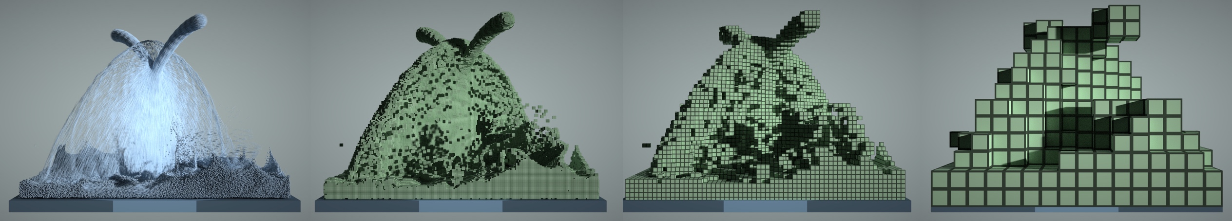 Figure: A 3D fluid simulation that uses both particles and grids. Left to right: particles, 1x1x1 voxels, 4x4x4 blocks, 16x16x16 blocks.
Motivation
In large-scale spatial computing, such as physical modelling, graphics, and 3D reconstruction, high-resolution 2D/3D grids are frequently required. However, if we employ dense data structures, these grids tend to consume a significant amount of memory space and processing (see field and field advanced). While a programmer may allocate large dense grids to store spatial data (particularly physical qualities such as a density or velocity field), they may only be interested in a tiny percentage of this dense grid because the remainder may be empty space (vacuum or air).
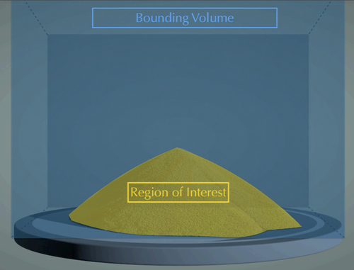
To illustrate this idea, the regions of interest in sparse grids shown below may only occupy a small fraction of the whole bounding box. If we can leverage such "spatial sparsity" and focus computation on the regions we care about, we will significantly save storage and computing power.
note
The key to leveraging spatial sparsity is replacing dense grids with sparse grids.
Sparse data structures are traditionally based on Quadtrees (2D) and Octrees (3D). Given that dereferencing pointers is relatively costly on modern computer architectures, Quadtrees and Octrees are less performance friendly than shallower trees with larger branching factors, such as VDB and SPGrid. In Taichi, you can compose data structures similar to VDB and SPGrid with SNodes. The advantages of Taichi spatially sparse data structures include:
- Access with indices, which just like accessing a dense data structure.
- Automatic parallelization when iterating.
- Automatic memory access optimization.
note
Backend compatibility: The LLVM-based backends (CPU/CUDA) offer the full functionality for performing computations on spatially sparse data structures. Using sparse data structures on the Metal backend is now deprecated. The support for Dynamic SNode has been removed in v1.3.0, and the support for Pointer/Bitmasked SNode will be removed in v1.4.0.
note
Sparse matrices are usually not implemented in Taichi via spatially sparse data structures. See sparse matrix instead.
Spatially sparse data structures in Taichi
Spatially sparse data structures in Taichi are composed of pointer, bitmasked, dynamic, and dense SNodes. A SNode tree merely composed of dense SNodes is not a spatially sparse data structure.
On a spatially sparse data structure, we consider a pixel, a voxel, or a grid node to be active if it is allocated and involved in the computation.
The rest of the grid simply becomes inactive.
In SNode terms, the activity of a leaf or intermediate cell is represented as a Boolean value. The activity value of a cell is True if and only if the cell is active. When writing to an inactive cell, Taichi automatically activates it. Taichi also provides manual manipulation of the activity of a cell: See Explicitly manipulating and querying sparsity.
note
Reading an inactive pixel returns zero.
Pointer SNode
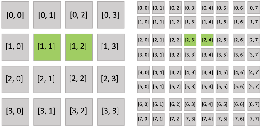
The code snippet below creates an 8x8 sparse grid, with the top-level being a 4x4 pointer array (line 2 of pointer.py),
and each pointer pointing to a 2x2 dense block.
Just as you do with a dense field, you can use indices to write and read the sparse field. The following figure shows the active blocks and pixels in green.
x = ti.field(ti.f32)
block = ti.root.pointer(ti.ij, (4,4))
pixel = block.dense(ti.ij, (2,2))
pixel.place(x)

@ti.kernel
def activate():
    x[2,3] = 1.0
    x[2,4] = 2.0

@ti.kernel
def print_active():
    for i, j in block:
        print("Active block", i, j)
    # output: Active block 1 1
    #         Active block 1 2
    for i, j in x:
        print('field x[{}, {}] = {}'.format(i, j, x[i, j]))
    # output: field x[2, 2] = 0.000000
    #         field x[2, 3] = 1.000000
    #         field x[3, 2] = 0.000000
    #         field x[3, 3] = 0.000000
    #         field x[2, 4] = 2.000000
    #         field x[2, 5] = 0.000000
    #         field x[3, 4] = 0.000000
    #         field x[3, 5] = 0.000000
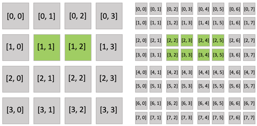
Executing the activate() function automatically activates block[1,1], which includes x[2,3], and block[1,2], which includes x[2,4]. Other pixels of block[1,1] (x[2,2], x[3,2], x[3,3]) and block[1,2] (x[2,5], x[3,4], x[3,5]) are also implicitly activated because all pixels in the dense block share the same activity value.
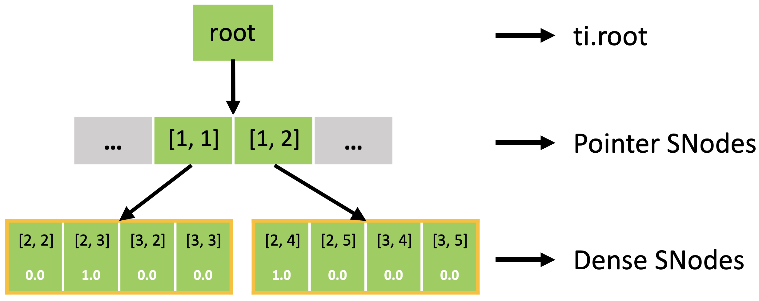
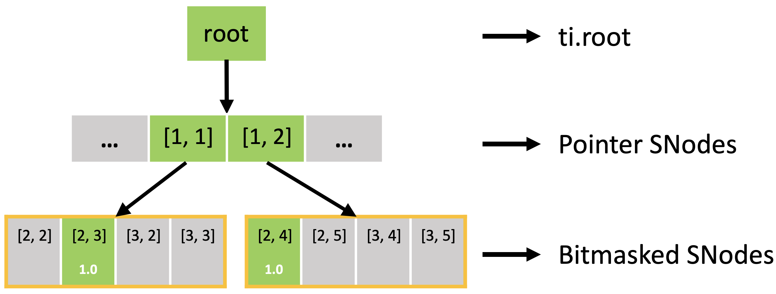
In fact, the sparse field is an SNode tree shown in the following figure. You can use a for loop to loop over the different levels of the SNode tree like the print_active() function in the previous example. A parallelized loop over a block for i, j in block would loop over all active pointer SNodes. A parallelized loop over a pixel for i, j in pixel would loop over all active dense SNodes.
Bitmasked SNode
While a null pointer can effectively represent an empty sub-tree, using 64 bits to represent the activity of a single pixel at the leaf level can consume too much space.
For example, if each pixel contains a single f32 value (4 bytes),
the 64-bit pointer pointing to the value would take 8 bytes.
The fact that storage costs of pointers are higher than the space to store the value themselves
goes against our goal to use spatially sparse data structures to save space.
To amortize the storage cost of pointers, you could organize pixels in a blocked manner
and let the pointers directly point to the blocks like the data structure defined in pointer.py.
One caveat of this design is that pixels in the same dense block can no longer change their activity flexibly.
Instead, they share a single activity flag. To address this issue,
the bitmasked SNode additionally allocates 1-bit per pixel data to represent the pixel activity.
The code snippet below illustrates this idea using a 8x8 grid. The only difference between bitmasked.py and pointer.py is that the bitmasked SNode replaces the dense SNode (line 3).
x = ti.field(ti.f32)
block = ti.root.pointer(ti.ij, (4,4))
pixel = block.bitmasked(ti.ij, (2,2))
pixel.place(x)

@ti.kernel
def activate():
    x[2,3] = 1.0
    x[2,4] = 2.0

@ti.kernel
def print_active():
    for i, j in block:
        print("Active block", i, j)
    for i, j in x:
        print('field x[{}, {}] = {}'.format(i, j, x[i, j]))
Furthermore, the active blocks are the same as pointer.py as shown below. However, the bitmasked pixels in the block are not all activated, because each of them has an activity value.
The bitmasked SNodes are like dense SNodes with auxiliary activity values.
Dynamic SNode
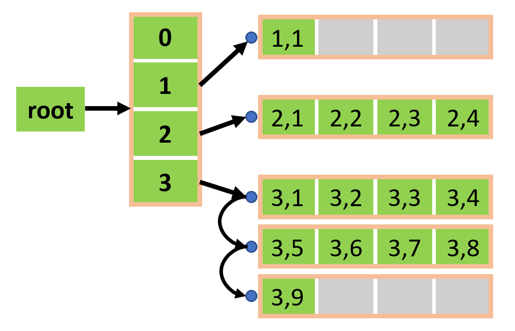
To support variable-length fields, Taichi provides dynamic SNodes.
The first argument of dynamic is the axis, the second argument is the maximum length,
and the third argument (optional) is the chunk_size.
The chunk_size specifies how much space the dynamic SNode allocates when the previously-allocated space runs out.
For example, with chunk_size=4, the dynamic SNode allocates the space for four elements when the first element is appended, and
allocates space for another four when the 5th (, 9th, 13th...) element is appended.
You can use x[i].append(...) to append an element,
use x[i].length() to get the length, and use x[i].deactivate() to clear the list.
The code snippet below creates a struct field that stores pairs of (i16, i64).
The i axis is a dense SNode, and the j axis is a dynamic SNode.
pair = ti.types.struct(a=ti.i16, b=ti.i64)
pair_field = pair.field()

block = ti.root.dense(ti.i, 4)
pixel = block.dynamic(ti.j, 100, chunk_size=4)
pixel.place(pair_field)
l = ti.field(ti.i32)
ti.root.dense(ti.i, 5).place(l)

@ti.kernel
def dynamic_pair():
    for i in range(4):
        pair_field[i].deactivate()
        for j in range(i * i):
            pair_field[i].append(pair(i, j + 1))
        # pair_field = [[],
        #              [(1, 1)],
        #              [(2, 1), (2, 2), (2, 3), (2, 4)],
        #              [(3, 1), (3, 2), ... , (3, 8), (3, 9)]]
        l[i] = pair_field[i].length()  # l = [0, 1, 4, 9]
note
A dynamic SNode must have one axis only, and the axis must be the last axis. No other SNodes can be placed under a dynamic SNode. In other words, a dynamic SNode must be directly placed with a field. Along the path from a dynamic SNode to the root of the SNode tree, other SNodes must not have the same axis as the dynamic SNode.
Computation on spatially sparse data structures
Sparse struct-fors
Efficiently looping over sparse grid cells that distribute irregularly can be challenging, especially on parallel devices such as GPUs.
In Taichi, for loops natively support spatially sparse data structures and only loop over currently active pixels with automatic efficient parallelization.
Explicitly manipulating and querying sparsity
Taichi also provides APIs that explicitly manipulate data structure sparsity. You can manually check the activity of a SNode, activate a SNode, or deactivate a SNode. We now illustrate these functions based on the field defined below.
x = ti.field(dtype=ti.i32)
block1 = ti.root.pointer(ti.ij, (3, 3))
block2 = block1.pointer(ti.ij, (2, 2))
pixel = block2.bitmasked(ti.ij, (2, 2))
pixel.place(x)
1. Activity checking
You can use ti.is_active(snode, [i, j, ...]) to explicitly query if snode[i, j, ...] is active or not.
@ti.kernel
def activity_checking(snode: ti.template(), i: ti.i32, j: ti.i32):
    print(ti.is_active(snode, [i, j]))

for i in range(3):
    for j in range(3):
        activity_checking(block1, i, j)
for i in range(6):
    for j in range(6):
        activity_checking(block2, i, j)
for i in range(12):
    for j in range(12):
        activity_checking(pixel, i, j)
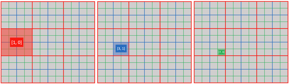
2. Activation
You can use ti.activate(snode, [i, j, ...]) to explicitly activate a cell of snode[i, j, ...].
@ti.kernel
def activate_snodes():
    ti.activate(block1, [1, 0])
    ti.activate(block2, [3, 1])
    ti.activate(pixel, [7, 3])

activity_checking(block1, 1, 0) # output: 1
activity_checking(block2, 3, 1) # output: 1
activity_checking(pixel, 7, 3)  # output: 1
3. Deactivation
- Use
ti.deactivate(snode, [i, j, ...])to explicitly deactivate a cell ofsnode[i, j, ...]. - Use
snode.deactivate_all()to deactivate all cells of SNodesnode. This operation also recursively deactivates all its children. - Use
ti.deactivate_all_snodes()to deactivate all cells of all SNodes with sparsity.
When deactivation happens, the Taichi runtime automatically recycles and zero-fills memory of the deactivated containers.
note
For performance reasons, ti.activate(snode, index) only activates snode[index].
The programmer must ensure that all ancestor containers of snode[index] is already active.
Otherwise, this operation results in undefined behavior.
Similarly, ti.deactivate ...
- does not recursively deactivate all the descendants of a cell.
- does not trigger deactivation of its parent container, even if all the children of the parent container are deactivated.
4. Ancestor index query
You can use ti.rescale_index(descendant_snode/field, ancestor_snode, index) to compute the ancestor index given a descendant index.
print(ti.rescale_index(x, block1, ti.Vector([7, 3]))) # output: [1, 0]
print(ti.rescale_index(x, block2, [7, 3]))            # output: [3, 1]
print(ti.rescale_index(x, pixel,  [7, 3]))            # output: [7, 3]
print(ti.rescale_index(block2, block1, [3, 1]))       # output: [1, 0]
Regarding line 1, you can also compute the block1 index given pixel index [7, 3] as [7//2//2, 3//2//2]. However, doing so couples computation code with the internal configuration of data structures (in this case, the size of block1 containers). By using ti.rescale_index(), you can avoid hard-coding internal information of data structures.
Further reading
Please read the SIGGRAPH Asia 2019 paper or watch the associated introduction video with slides for more details on computation of spatially sparse data structures.
Taichi elements implement a high-performance MLS-MPM solver on Taichi sparse grids.