Fields (advanced)
Modern processor cores compute orders of magnitude faster than their equipped memory systems. To shrink this performance gap, multi-level cache systems and high-bandwidth multi-channel memories are built into the computer architectures.
After familiarizing yourself with the basics of Taichi Fields, this article helps you one step further by explaining the underlying memory layout that is essential to write high-performance Taichi programs. In particular, we present how to organize an efficient data layout and how to manage memory occupancy.
Organizing an efficient data layout
In this section, we introduce how to organize data layouts in Taichi fields. The central principle of efficient data layout is locality. Generally speaking, a program with desirable locality has at least one of the following features:
- Dense data structures
- Small-range data looping (within 32KB is good for most processors)
- Sequentially loading and storing data
note
Be aware that data is traditionally fetched from memory in blocks (pages). In addition, the hardware itself has little knowledge about how a specific data element is used in the block. The processor blindly fetches the entire block according to the requested memory address. Thus, the memory bandwidth is wasted when data are not fully utilized.
For sparse fields, see the Sparse computation.
Layout 101: from shape to ti.root.X
In basic usages, we use the shape descriptor to construct a field. Taichi provides flexible statements to describe more advanced data organizations, the ti.root.X.
Here are some examples:
- Declare a 0-D field:
x = ti.field(ti.f32)
ti.root.place(x)

# is equivalent to:
x = ti.field(ti.f32, shape=())
- Declare a 1-D field of shape
3:
x = ti.field(ti.f32)
ti.root.dense(ti.i, 3).place(x)

# is equivalent to:
x = ti.field(ti.f32, shape=3)
- Declare a 2-D field of shape
(3, 4):
x = ti.field(ti.f32)
ti.root.dense(ti.ij, (3, 4)).place(x)
# is equivalent to:
x = ti.field(ti.f32, shape=(3, 4))
You can also nest two 1D dense statements to describe a 2D array of the same shape.
x = ti.field(ti.f32)
ti.root.dense(ti.i, 3).dense(ti.j, 4).place(x)
# has the same shape with
x = ti.field(ti.f32, shape=(3,4))
note
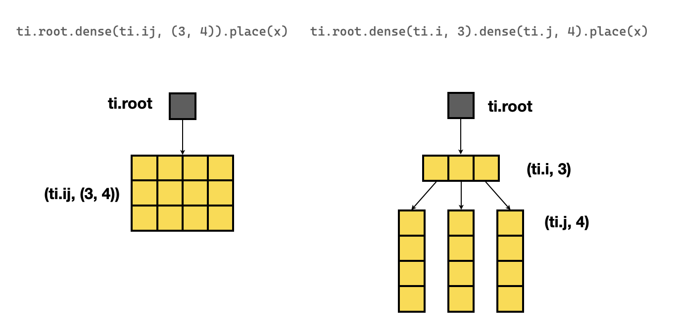
The above 2D array built with nested dense statements is not equivalent to the 2D array built with ti.field.
Although both statements result in a 2D array of the same shape, they have
different layers of SNodeTree, as shown below:
The following snippet has two SNodeTree layers below the root:
x = ti.field(ti.f32)
ti.root.dense(ti.i, 3).dense(ti.j, 4).place(x)
The following snippet only has one SNodeTree below the root:
x = ti.field(ti.f32)
ti.root.dense(ti.ij, (3, 4)).place(x)

# or equivalently
x = ti.field(ti.f32, shape=(3,4))
See the sketch below for a visualization that illustrates the difference between these layers:
The difference here is subtle as both arrays are row-major, but it may have slight performance impact
because the overhead of calculating the SNodeTree index is different for the two.
In a nutshell, the ti.root.X statement progressively binds a shape to the corresponding axis.
By nesting multiple statements, we can construct a field with higher dimensions.
In order to traverse the nested statements, you can use a for loop:
for i, j in A:
    A[i, j] += 1
The Taichi compiler is capable of automatically deducing the underlying data layout and applying a proper data access order. This is an advantage over most general-purpose programming languages where the access order has to be optimized manually.
Row-major versus column-major
One important thing to note about memory addresses is that their space is linear. Without loss of generality, we omit the differences in data types and assume each data element has size 1. Moreover, we denote the starting memory address of a field as base, and the indexing formula for 1D Taichi fields is base + i for the i-th element.
For multi-dimensional fields, we can flatten the high-dimension index into the linear memory address space in two ways: Taking a 2D field of shape (M, N) as an instance, we can either store M rows with N-length 1D buffers, say the row-major way, or store N columns, say the column-major way. The index flatten formula for the (i, j)-th element is base + i * N + j for row-major and base + j * M + i for column-major, respectively.
Trivially, elements in the same row are close in memory for row-major fields. The selection of the optimal layout is based on how the elements are accessed, namely, the access patterns. Patterns such as frequently accessing elements of the same row in a column-major field typically lead to performance degradation.
The default Taichi field layout is row-major. With the ti.root statements, fields can be defined as follows:
x = ti.field(ti.f32)
y = ti.field(ti.f32)
ti.root.dense(ti.i, M).dense(ti.j, N).place(x)   # row-major
ti.root.dense(ti.j, N).dense(ti.i, M).place(y)   # column-major
In the code above, the axis denotation in the rightmost dense statement indicates the continuous axis. For the x field, elements in the same row (with same i and different j) are close in memory, hence it's row-major; For the y field, elements in the same column (same j and different i) are close, hence it's column-major. With an example of (2, 3), we visualize the memory layouts of x and y as follows:
# address:  low ........................................... high
#       x:  x[0, 0]  x[0, 1]  x[1, 0]  x[1, 1]  x[2, 0]  x[2, 1]
#       y:  y[0, 0]  y[1, 0]  y[2, 0]  y[0, 1]  y[1, 1]  y[2, 1]
It is worth noting that the accessor is unified for Taichi fields: the (i, j)-th element in the field is accessed with the identical 2D index x[i, j] and y[i, j]. Taichi handles the layout variants and applies proper indexing equations internally. Thanks to this feature, users can specify their desired layout at definition, and use the fields without concerning about the underlying memory organizations. To change the layout, we can simply swap the order of dense statements, and leave rest of the code intact.
note
For readers who are familiar with C/C++, below is an example C code snippet that demonstrates data access in 2D arrays:
int x[3][2];  // row-major
int y[2][3];  // column-major

for (int i = 0; i < 3; i++) {
    for (int j = 0; j < 2; j++) {
        do_something(x[i][j]);
        do_something(y[j][i]);
    }
}
The accessors of x and y are in reverse order between row-major arrays and column-major arrays, respectively. Compared with Taichi fields, there is much more code to revise when you change the memory layout.
AoS versus SoA
AoS means array of structures and SoA means structure of arrays. Consider an RGB image with four pixels and three color channels: an AoS layout stores RGBRGBRGBRGB while an SoA layout stores RRRRGGGGBBBB. The selection of an AoS or SoA layout largely depends on the access pattern to the field. Let's discuss a scenario to process large RGB images. The two layouts have the following arrangements in memory:
# address: low ...................... high
# AoS:     RGBRGBRGBRGBRGBRGB.............
# SoA:     RRRRR...RGGGGGGG...GBBBBBBB...B
To calculate grey scale of each pixel, you need all color channels but do not require the value of other pixels. In this case, the AoS layout has a better memory access pattern: Since color channels are stored continuously, and adjacent channels can be fetched instantly. The SoA layout is not a good option because the color channels of a pixel are stored far apart in the memory space.
We describe how to construct AoS and SoA fields with our ti.root.X statements. The SoA fields are trivial:
x = ti.field(ti.f32)
y = ti.field(ti.f32)
ti.root.dense(ti.i, M).place(x)
ti.root.dense(ti.i, M).place(y)
where M is the length of x and y.
The data elements in x and y are continuous in memory:
#  address: low ................................. high
#           x[0]  x[1]  x[2] ... y[0]  y[1]  y[2] ...
For AoS fields, we construct the field with
x = ti.field(ti.f32)
y = ti.field(ti.f32)
ti.root.dense(ti.i, M).place(x, y)
The memory layout then becomes
#  address: low .............................. high
#           x[0]  y[0]  x[1]  y[1]  x[2]  y[2] ...
Here, place interleaves the elements of Taichi fields x and y.
As previously introduced, the access methods to x and y remain the same for both AoS and SoA. Therefore, the data layout can be changed flexibly without revising the application logic.
For better illustration, let's see an example of an 1D wave equation solver:
N = 200000
pos = ti.field(ti.f32)
vel = ti.field(ti.f32)
# SoA placement
ti.root.dense(ti.i, N).place(pos)
ti.root.dense(ti.i, N).place(vel)

@ti.kernel
def step():
    pos[i] += vel[i] * dt
    vel[i] += -k * pos[i] * dt
The above code snippet defines SoA fields and a step kernel that sequentially accesses each element.
The kernel fetches an element from pos and vel for every iteration, respectively.
For SoA fields, the closest distance of any two elements in memory is N, which is unlikely to be efficient for large N.
We hereby switch the layout to AoS as follows:
N = 200000
pos = ti.field(ti.f32)
vel = ti.field(ti.f32)
# AoS placement
ti.root.dense(ti.i, N).place(pos, vel)

@ti.kernel
def step():
    pos[i] += vel[i] * dt
    vel[i] += -k * pos[i] * dt
Merely revising the place statement is sufficient to change the layout. With this optimization, the instant elements pos[i] and vel[i] are now adjacent in memory, which is more efficient.
AoS extension: hierarchical fields
Sometimes we want to access memory in a complex but fixed pattern, like traversing an image in 8x8 blocks. The apparent best practice is to flatten each 8x8 block and concatenate them together. However, the field is no longer a flat buffer as it now has a hierarchy with two levels: The image level and the block level. Equivalently, the field is an array of implicit 8x8 block structures.
We demonstrate the statements as follows:
# Flat field
val = ti.field(ti.f32)
ti.root.dense(ti.ij, (M, N)).place(val)
# Hierarchical field
val = ti.field(ti.f32)
ti.root.dense(ti.ij, (M // 8, N // 8)).dense(ti.ij, (8, 8)).place(val)
where M and N are multiples of 8. We encourage you to try this out! The performance difference can be significant!
note
We highly recommend that you use power-of-two block size so that accelerated indexing with bitwise arithmetic and better memory address alignment can be enabled.
Manage memory occupancy
Manual field allocation and destruction
Generally, Taichi manages memory allocation and destruction without disturbing the users. However, there are times that users want explicit control over their memory allocations.
In this scenario, Taichi provides the FieldsBuilder for manual field memory allocation and destruction. FieldsBuilder features identical declaration APIs as ti.root. The extra step is to invoke finalize() at the end of all declarations. The finalize() returns an SNodeTree object to handle subsequent destructions.
Let's see a simple example:
import taichi as ti
ti.init()

@ti.kernel
def func(v: ti.template()):
    for I in ti.grouped(v):
        v[I] += 1

fb1 = ti.FieldsBuilder()
x = ti.field(dtype=ti.f32)
fb1.dense(ti.ij, (5, 5)).place(x)
fb1_snode_tree = fb1.finalize()  # Finalizes the FieldsBuilder and returns a SNodeTree
func(x)
fb1_snode_tree.destroy()  # Destruction

fb2 = ti.FieldsBuilder()
y = ti.field(dtype=ti.f32)
fb2.dense(ti.i, 5).place(y)
fb2_snode_tree = fb2.finalize()  # Finalizes the FieldsBuilder and returns a SNodeTree
func(y)
fb2_snode_tree.destroy()  # Destruction
The above demonstrated ti.root statements are implemented with FieldsBuilder, despite that ti.root has the capability to automatically manage memory allocations and recycling.